
// 퇴근후딴짓 님의 강의를 참고하였습니다. //
Dataset :
문제) 신용카드 서비스를 떠나는 고객을 찾아라.
- 나이, 급여, 결혼 상태, 신용 카드 한도, 신용 카드 카테고리 등의 컬럼이 있음.
- 평가: ROC-AUC, 정확도(Accuracy), F1, 정밀도(Precision), 재현율(Recall)을 구하시오.
- target : Attrition_Flag (1:이탈, 0:유지)
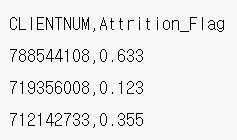
- csv파일 생성 : 수험번호.csv (예시 아래 참조)
1. 데이터 불러오기
import pandas as pd

train = pd.read_csv("train.csv")
test =  pd.read_csv("test.csv")
→ train과 test 2개의 파일로 나누어져있다.
2. EDA
train.shape, test.shape

실행 결과 :
(8101, 21) (2026, 20)
train.head()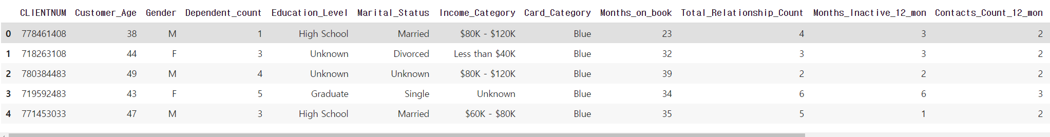
→ train 데이터는 21개의 열로 이루어져있다.
test.head()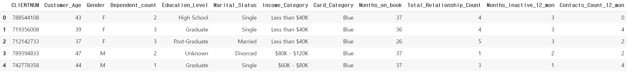
→ test 데이터는 20개의 열로 이루어져있다.
train.info()

실행 결과 :
<class 'pandas.core.frame.DataFrame'>
RangeIndex: 8101 entries, 0 to 8100
Data columns (total 21 columns):
 #   Column                    Non-Null Count  Dtype
---  ------                    --------------  -----
 0   CLIENTNUM                 8101 non-null   int64
 1   Customer_Age              8101 non-null   int64
 2   Gender                    8101 non-null   object
 3   Dependent_count           8101 non-null   int64
 4   Education_Level           8101 non-null   object
 5   Marital_Status            8101 non-null   object
 6   Income_Category           8101 non-null   object
 7   Card_Category             8101 non-null   object
 8   Months_on_book            8101 non-null   int64
 9   Total_Relationship_Count  8101 non-null   int64
 10  Months_Inactive_12_mon    8101 non-null   int64
 11  Contacts_Count_12_mon     8101 non-null   int64
 12  Credit_Limit              8101 non-null   float64
 13  Total_Revolving_Bal       8101 non-null   int64
 14  Avg_Open_To_Buy           8101 non-null   float64
 15  Total_Amt_Chng_Q4_Q1      8101 non-null   float64
 16  Total_Trans_Amt           8101 non-null   int64
 17  Total_Trans_Ct            8101 non-null   int64
 18  Total_Ct_Chng_Q4_Q1       8101 non-null   float64
 19  Avg_Utilization_Ratio     8101 non-null   float64
 20  Attrition_Flag            8101 non-null   int64
dtypes: float64(5), int64(11), object(5)
→ 5개의 실수형, 11개의 정수형, 5개의 object형으로 이루어져있다.
train['Attrition_Flag'].value_counts()

실행 결과 :
0    6815
1    1286
Name: Attrition_Flag, dtype: int64
→ target으로 사용할 'Attrition_Flag' 열은 유지(0) 6815건, 이탈(1) 1286건으로 이루어져있다.
→ 이렇게 데이터 불균형이 있을경우 모델의 성능이 좋지 않을수도 있다.
train.isnull().sum()

실행 결과 :
CLIENTNUM                   0
Customer_Age                0
Gender                      0
Dependent_count             0
Education_Level             0
Marital_Status              0
Income_Category             0
Card_Category               0
Months_on_book              0
Total_Relationship_Count    0
Months_Inactive_12_mon      0
Contacts_Count_12_mon       0
Credit_Limit                0
Total_Revolving_Bal         0
Avg_Open_To_Buy             0
Total_Amt_Chng_Q4_Q1        0
Total_Trans_Amt             0
Total_Trans_Ct              0
Total_Ct_Chng_Q4_Q1         0
Avg_Utilization_Ratio       0
Attrition_Flag              0
dtype: int64
test.isnull().sum()
실행 결과 :
CLIENTNUM 0
Customer_Age 0
Gender 0
Dependent_count 0
Education_Level 0
Marital_Status 0
Income_Category 0
Card_Category 0
Months_on_book 0
Total_Relationship_Count 0
Months_Inactive_12_mon 0
Contacts_Count_12_mon 0
Credit_Limit 0
Total_Revolving_Bal 0
Avg_Open_To_Buy 0
Total_Amt_Chng_Q4_Q1 0
Total_Trans_Amt 0
Total_Trans_Ct 0
Total_Ct_Chng_Q4_Q1 0
Avg_Utilization_Ratio 0
dtype: int64→ train, test 데이터 모두 결측치는 없다.
3. 데이터 전처리 & 피처엔지니어링
→ label 작업 여부에 따른 결과를 비교해 볼 예정이다.
# 기본 / label x
cols = train.select_dtypes(include='object').columns
cols

print(train.shape, test.shape)
train = train.drop(cols, axis=1)
test = test.drop(cols, axis=1)
print(train.shape, test.shape)

# train.drop(cols, axis=1, inplace=True)

실행 결과 :
(8101, 21) (2026, 20)
(8101, 16) (2026, 15)
→ train, test 데이터의 object형 컬럼을 제거한 후의 컬럼 개수이다. 5개씩 감소하였다.
→ drop 파라미터에서 inplace=True를 하면 변수에 담지 않아도 바로 제거가 적용된다.
# label
from sklearn.preprocessing import LabelEncoder

for col in cols:
	le = LabelEncoder()
	train[col] = le.fit_transform(train[col])
    test[col] = le.transform(test[col])
→ object 컬럼들을 label 작업하는 코드이다.
train = train.drop('CLIENTNUM', axis=1)
test_id = test.pop('CLIENTNUM')
→ 제출파일에서 id로 사용될 'CLIENTNUM' 컬럼을 제거 및 test_id 변수에 따로 담아둔다.
4. 검증 데이터 분리
from sklearn.model_selection import train_test_split

X_tr, X_val, y_tr, y_val = train_test_split(
    train.drop('Attrition_Flag', axis=1), train['Attrition_Flag'], test_size=0.2, random_state=2022
)
→ target 컬럼인 'Attrition_Flag' 를 train에서는 제거하고 test에서는 'Attrition_Flag' 컬럼만 포함시켜 분리한다.
5. 모델 & 평가
from sklearn.ensemble import RandomForestClassifier

model = RandomForestClassifier(random_state=2022)
model.fit(X_tr, y_tr)
pred = model.predict(X_val)
→ 랜덤포레스트 모델로 훈련시킨 후 예측하는 코드이다.
from sklearn.metrics import accuracy_score, precision_score, recall_score, f1_score, roc_auc_score

# 정확도
print(accuracy_score(y_val, pred))

# 정밀도
print(precision_score(y_val, pred))

# 재현율 (민감도)
print(recall_score(y_val, pred))

# F1
print(f1_score(y_val , pred))

# baseline
# 0.9666872301048736
# 0.9444444444444444
# 0.8435114503816794
# 0.8911290322580645
# 0.8716904276985744

# label
# 0.9685379395434917
# 0.948936170212766
# 0.851145038167939
# 0.89738430583501
# 0.8716904276985744
→ 정확도, 정밀도, 재현율, f1_score로 평가한 결과이다.
→ object 컬럼을 삭제하는것보다 label 작업 후 모델을 훈련 시킨것이 점수가 미세하게 더 높게 나왔다.
# roc-auc
pred = model.predict_proba(X_val)
print(roc_auc_score(y_val, pred[:,1]))

# baseline
# 0.9894048160692921

# label
# 0.9899707351049547
→ roc_auc_score로 평가한 결과이다.
→ roc_auc_score로 평가시에는 predict 대신 predict_proba를 사용하여 확률을 구해야한다.
→ roc_auc_score 또한 label 작업한 것이 점수하게 미세하게 높게 나왔다.
6. 예측 및 csv 제출
pred = model.predict_proba(test)
pred

실행 결과 :
array([[1.  , 0.  ],
       [0.98, 0.02],
       [0.93, 0.07],
       ...,
       [0.8 , 0.2 ],
       [0.99, 0.01],
       [0.98, 0.02]])
→ 검증용 데이터가 아닌 실제 제출용 test 데이터로 예측한 결과이다.
→ array 왼쪽은 유지 확률, 오른쪽은 이탈 확률을 나타낸다.
submit = pd.DataFrame({
    'CLIENTNUM':test_id,
    'Attrition_Flag':pred[:,1]
})
submit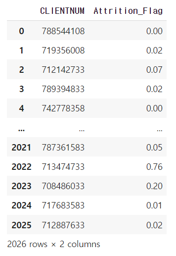
→ 문제 예시와 같이 'CLIENTNUM' 컬럼에 test_id를 'Attrition_Flag' 컬럼에 이탈 확률을 넣어 데이터프레임을 만든다.
submit.to_csv('00000.csv', index=False)→ 데이터프레임을 제출용 csv 파일로 만든다. index는 제거한다.
pd.read_csv("00000.csv")→ 제출용 csv 파일을 만든 후 read_csv로 불러와 제출이 제대로 되었는지 재확인한다.
'빅데이터분석기사 > 작업형2' 카테고리의 다른 글
| [작업형2] 심장마비 확률 높은 사람 구하기(분류 / 튜닝) (0) | 2023.06.17 |
|---|---|
| [작업형2] 에어비앤비 가격 예측하기(회귀) (0) | 2023.06.17 |
| [작업형2] 보험가입 확률 구하기(분류) (1) | 2023.06.17 |
| [작업형2] 제품 배송 시간에 맞춰 배송되었는지 예측하기(분류) (0) | 2023.06.15 |
| [작업형2] 고객의 성별이 남자일 확률 구하기(분류) (1) | 2023.06.15 |