
// 퇴근후딴짓 님의 강의를 참고하였습니다. //
Dataset :
문제) 심장마비 확률이 높은 사람을 다음과 같은 형식의 CSV 파일로 생성하시오.
- 성별, 나이, 혈압, 콜레스테롤, 공복혈당, 최대 심박수 등의 컬럼이 있음.
- 평가: ROC-AUC, 정확도(Accuracy), F1 을 구하시오.
- target : output (1:심장마비 확률 높음, 0:심장마비 확률 낮음)
- csv파일 생성 : 수험번호.csv (예시 아래 참조)
1. 데이터 불러오기
import pandas as pd

train = pd.read_csv("train.csv")
test =  pd.read_csv("test.csv")
print(train.shape, test.shape)

실행 결과 :
(242, 15) (61, 14)
→ train과 test 2개의 파일로 나누어져있다.
→ train 데이터는 15개의 열로 이루어져있다.
→ test 데이터는 14개의 열로 이루어져있다.
2. EDA
train.head(2)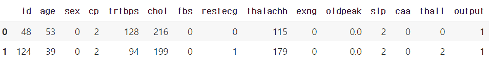
test.head(2)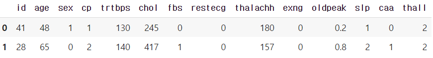
→ target 컬럼인 'output' 컬럼이 train 데이터에만 있다.
train['output'].value_counts()

실행 결과 :
1    126
0    116
Name: output, dtype: int64
→ target으로 사용할 'output' 열은 낮음(0) 116건, 높음(1) 126건으로 이루어져있다.
train.isnull().sum()

실행 결과 :
id          0
age         0
sex         0
cp          0
trtbps      0
chol        0
fbs         0
restecg     0
thalachh    0
exng        0
oldpeak     0
slp         0
caa         0
thall       0
output      0
dtype: int64
test.isnull().sum()
실행 결과 :
id 0
age 0
sex 0
cp 0
trtbps 0
chol 0
fbs 0
restecg 0
thalachh 0
exng 0
oldpeak 0
slp 0
caa 0
thall 0
dtype: int64→ train, test 데이터 모두 결측치는 없다.
train.describe()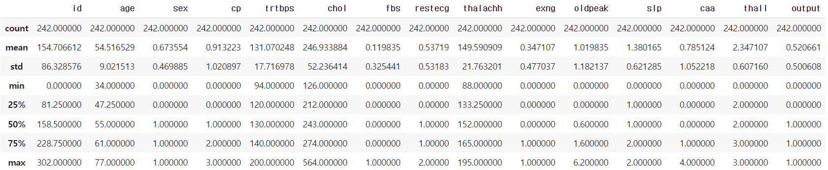
→ train 데이터의 기초통계량이다.
train.info()

실행 결과 :
<class 'pandas.core.frame.DataFrame'>
RangeIndex: 242 entries, 0 to 241
Data columns (total 15 columns):
 #   Column    Non-Null Count  Dtype
---  ------    --------------  -----
 0   id        242 non-null    int64
 1   age       242 non-null    int64
 2   sex       242 non-null    int64
 3   cp        242 non-null    int64
 4   trtbps    242 non-null    int64
 5   chol      242 non-null    int64
 6   fbs       242 non-null    int64
 7   restecg   242 non-null    int64
 8   thalachh  242 non-null    int64
 9   exng      242 non-null    int64
 10  oldpeak   242 non-null    float64
 11  slp       242 non-null    int64
 12  caa       242 non-null    int64
 13  thall     242 non-null    int64
 14  output    242 non-null    int64
dtypes: float64(1), int64(14)
→ 1개의 실수형, 14개의 정수형 컬럼으로 이루어져있다.
train.nunique()

실행 결과 :
id          242
age          40
sex           2
cp            4
trtbps       47
chol        139
fbs           2
restecg       3
thalachh     83
exng          2
oldpeak      38
slp           3
caa           5
thall         4
output        2
dtype: int64
→ 각 열의 카테고리 개수이다.
3. 데이터 전처리 & 피처엔지니어링
train = train.drop('id', axis=1)
test_id = test.pop('id')
→ 제출파일에서 id로 사용될 'id' 컬럼을 제거 및 test_id 변수에 따로 담아둔다.
4. 검증 데이터 분리
from sklearn.model_selection import train_test_split
X_tr, X_val, y_tr, y_val = train_test_split(train.drop('output', axis=1), train['output'],
                                            test_size=0.15, random_state=2022)
→ target 컬럼인 'output' 를 train에서는 제거하고 test에서는 'output' 컬럼만 포함시켜 분리한다.
5. 모델 & 평가
# rf
from sklearn.ensemble import RandomForestClassifier
from sklearn.metrics import roc_auc_score, f1_score, accuracy_score

rf = RandomForestClassifier(random_state=2022, max_depth=5, n_estimators=400)
rf.fit(X_tr, y_tr)
pred = rf.predict(X_val)
pred_proba = rf.predict_proba(X_val)

print(roc_auc_score(y_val, pred_proba[:,1]))
print(f1_score(y_val, pred))
print(accuracy_score(y_val, pred))

# max_depth=3~12
# n_estimators=100 200 400 800 1000

# 0.9301242236024845
# 0.7906976744186046
# 0.7567567567567568

# max_depth=3
# 0.9378881987577639
# 0.8636363636363636
# 0.8378378378378378

# max_depth=5
# 0.9409937888198757
# 0.8444444444444444
# 0.8108108108108109

# max_depth=5, n_estimators=200
# 0.9440993788819876
# 0.8444444444444444
# 0.8108108108108109
→ 랜덤포레스트 모델로 max_depth, n_estimators 파라미터를 조정하면서 평가한 결과이다.
→ max_depth=5, n_estimators=200일때 가장 높은 점수가 나왔다.
→ max_depth는 3~12, n_estimators는 100~1000 사이로 튜닝하는게 일반적이다.
# xgb
from xgboost import XGBClassifier
xgb = XGBClassifier(random_state=2022, max_depth=5, n_estimators=600, learning_rate=0.01)
xgb.fit(X_tr, y_tr)
pred = xgb.predict(X_val)
pred_proba = xgb.predict_proba(X_val)

print(roc_auc_score(y_val, pred_proba[:,1]))
print(f1_score(y_val, pred))
print(accuracy_score(y_val, pred))

# max_depth 3 4 5 6 7 8 9 12
# n_estimators 100 ~ 1000
# learning_rate 0.1 ~ 0.01

# 0.9068322981366459
# 0.8444444444444444
# 0.8108108108108109

# max_depth=5
# 0.9130434782608695
# 0.8444444444444444
# 0.8108108108108109

# max_depth=5, n_estimators=400, learning_rate=0.01
# 0.9161490683229814
# 0.8372093023255814
# 0.8108108108108109

# max_depth=5, n_estimators=600, learning_rate=0.01
# 0.9192546583850931
# 0.8181818181818182
# 0.7837837837837838
→ xgboost 모델로 max_depth, n_estimators, learning_rate 파라미터를 조정하면서 평가한 결과이다.
→ max_depth=5, n_estimators=600, learning_rate=0.01일때 가장 높은 점수가 나왔다.
→ max_depth는 3~12, n_estimators는 100~1000, learning_rate는 0.1~0.01 사이로 튜닝하는게 일반적이다.
→ xgboost에서 n_estimators를 높이면 learning_rate는 낮춰줘야한다.
6. 예측 및 csv 제출
pred_proba = xgb.predict_proba(test)→ 검증용 데이터가 아닌 실제 제출용 test 데이터로 예측한 확률이다.
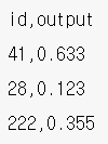
pd.DataFrame({'id':test_id, 'output':pred_proba[:,1]}).to_csv("00000.csv", index=False)→ 문제 예시와 같이 'id' 컬럼에 test_id를 'output' 컬럼에 심장마비 확률을 넣어 데이터프레임을 만든다.
pd.read_csv("00000.csv")→ 제출용 csv 파일을 만든 후 read_csv로 불러와 제출이 제대로 되었는지 재확인한다.
'빅데이터분석기사 > 작업형2' 카테고리의 다른 글
| [작업형2] 자동차 시장 세분화(분류) (0) | 2023.06.24 |
|---|---|
| [작업형2] 유방암 예측 모델 만들기(분류) (0) | 2023.06.22 |
| [작업형2] 에어비앤비 가격 예측하기(회귀) (0) | 2023.06.17 |
| [작업형2] 신용카드 서비스를 떠나는 고객 확률 구하기(분류) (0) | 2023.06.17 |
| [작업형2] 보험가입 확률 구하기(분류) (1) | 2023.06.17 |