
// 퇴근후딴짓 님의 강의를 참고하였습니다. //
Dataset :
문제) 제품 배송 시간에 맞춰 배송되었는지 예측모델 만들기(정시 도착하지 않을 확률), 다음과 같은 형식의 CSV 파일로 생성하시오.
- ID : 고객 ID
- Reached.on.Time_Y.N : 정시 도착 여부 (0: 정시 도착, 1: 정시 도착하지 않음)
1. 데이터 불러오기
# 시험환경 세팅 3개 파일 생성 (코드 변경 X)
import pandas as pd
import numpy as np
from sklearn.model_selection import train_test_split

def exam_data_load(df, target, id_name="", null_name=""):
    if id_name == "":
        df = df.reset_index().rename(columns={"index": "id"})
        id_name = 'id'
    else:
        id_name = id_name

    if null_name != "":
        df[df == null_name] = np.nan

    X_train, X_test = train_test_split(df, test_size=0.2, random_state=2022)
    y_train = X_train[[id_name, target]]
    X_train = X_train.drop(columns=[target])

    y_test = X_test[[id_name, target]]
    X_test = X_test.drop(columns=[target])
    return X_train, X_test, y_train, y_test

df = pd.read_csv("Train.csv") # 파일명이 다를 경우 파일명을 수정해주세요
X_train, X_test, y_train, y_test = exam_data_load(df, target='Reached.on.Time_Y.N', id_name='ID')
X_train.to_csv("X_train.csv", index=False)
y_train.to_csv("y_train.csv", index=False)
X_test.to_csv("X_test.csv", index=False)
→ Dataset이 Train.csv 1개로 합쳐져 있는 것을 나눠주는 코드이다.
# 데이터 불러오기
import pandas as pd
X_test = pd.read_csv("X_test.csv")
X_train = pd.read_csv("X_train.csv")
y_train = pd.read_csv("y_train.csv")

X_train.shape, y_train.shape, X_test.shape

실행 결과 :
((8799, 11), (8799, 2), (2200, 11))
2. EDA
# 데이터 확인(X_train)
X_train.head()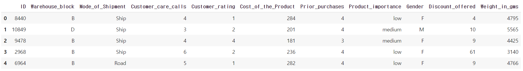
→ X_train은ID, Warehouse_block, Mode_of_shipment 등 11개의 열로 이루어져있다.
# 데이터 확인(y_train)
y_train.head()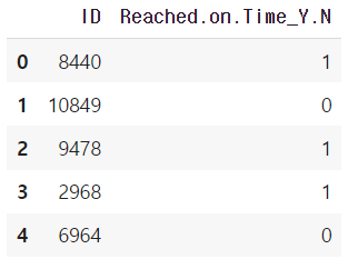
→ y_train은 ID와 Reached.on.Time_Y.N 2개의 열로 이루어져있다.
# 결측치 확인 train
X_train.isnull().sum()

실행 결과 :
ID                     0
Warehouse_block        0
Mode_of_Shipment       0
Customer_care_calls    0
Customer_rating        0
Cost_of_the_Product    0
Prior_purchases        0
Product_importance     0
Gender                 0
Discount_offered       0
Weight_in_gms          0
dtype: int64
→ X_train에는 결측치가 없다.
# 결측치 확인 test
X_test.isnull().sum()

실행 결과 :
ID                     0
Warehouse_block        0
Mode_of_Shipment       0
Customer_care_calls    0
Customer_rating        0
Cost_of_the_Product    0
Prior_purchases        0
Product_importance     0
Gender                 0
Discount_offered       0
Weight_in_gms          0
dtype: int64
→ X_test 또한 결측치가 없다.
# 타겟(레이블) 확인 0:정시 도착, 1: 정시 도착하지 않음
y_train['Reached.on.Time_Y.N'].value_counts()

실행 결과 :
1    5236
0    3563
Name: Reached.on.Time_Y.N, dtype: int64
→ y_train 확인 시 0이 3563, 1이 5236으로 정시 도착하지 않은 경우가 더 많은 것을 알 수 있다.
# 데이터 타입 확인
X_train.info()

실행 결과 :
<class 'pandas.core.frame.DataFrame'>
RangeIndex: 8799 entries, 0 to 8798
Data columns (total 11 columns):
 #   Column               Non-Null Count  Dtype
---  ------               --------------  -----
 0   ID                   8799 non-null   int64
 1   Warehouse_block      8799 non-null   object
 2   Mode_of_Shipment     8799 non-null   object
 3   Customer_care_calls  8799 non-null   int64
 4   Customer_rating      8799 non-null   int64
 5   Cost_of_the_Product  8799 non-null   int64
 6   Prior_purchases      8799 non-null   int64
 7   Product_importance   8799 non-null   object
 8   Gender               8799 non-null   object
 9   Discount_offered     8799 non-null   int64
 10  Weight_in_gms        8799 non-null   int64
dtypes: int64(7), object(4)
memory usage: 756.3+ KB
→ X_train은 7개의 수치형 변수와 4개의 명목형 변수로 이루어져있다.
# 기초 통계 획인
X_train.describe()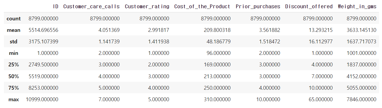
→ X_train 기초 통계 확인 시 특이사항은 보이지 않는다.
# X_train 기초 통계 확인 object
X_train.describe(include='object')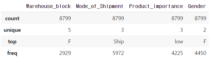
→ X_train의 명목형 변수는 Warehouse_block, Mode_of_Shipment, Product_importance, Gender 4가지 이다.
# X_test 기초 통계 획인 object
X_test.describe(include='object')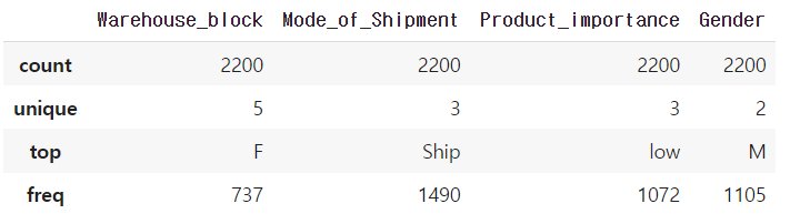
→ X_test의 명목형 변수 또한 Warehouse_block, Mode_of_Shipment, Product_importance, Gender 4가지 이다.
# [Tip] object 타입 고유값 개수 확인
X_train[['Warehouse_block', 'Mode_of_Shipment', 'Product_importance', 'Gender']].nunique()

실행 결과 :
Warehouse_block       5
Mode_of_Shipment      3
Product_importance    3
Gender                2
dtype: int64
→ object 타입의 고유값 개수를 물어 볼때 .nunique() 함수를 사용해 나타낼 수 있다.
# X데이터와 y데이터 합치기
df = pd.concat([X_train, y_train['Reached.on.Time_Y.N']], axis=1)
df.head(1)
→ pd.concat 함수를 사용해 X_train과 y_train의 Reached.on.Time_Y.N 열을 합쳐본다.
# idea? 할인율이 도착에 영향을 미칠까?
cond = df['Discount_offered'] > 5
sum(cond)

실행 결과 :
5480

cond = df['Discount_offered'] > 10
sum(cond)

실행 결과 :
2104
sum(df[cond]['Reached.on.Time_Y.N'])

실행 결과 :
3673

실행 결과 :
2104
→ 할인율이 도착에 영향을 미치는지 알아보기 위한 코드이다.
→ 할인율이 5프로 이상인 경우가 5480건일 때 정시에 도착하지 않은 경우는 3673건이다.
→ 할인율이 10프로 이상인 경우가 2104건일 때 정시에 도착하지 않은 경우는 2104건으로 100%이다.
→ 이는 할인율이 높을 수록 주문 배송이 많아 정시에 도착하지 않을 확률이 높았지 않을까라는 예측할 수 있다.
3. 데이터 전처리 및 피처엔지니어링
# 라벨 인코딩
from sklearn.preprocessing import LabelEncoder

cols = X_train.select_dtypes(include='object').columns
print(cols)

for col in cols:
  le = LabelEncoder()
  X_train[col] = le.fit_transform(X_train[col])
  X_test[col] = le.transform(X_test[col])

X_train.head()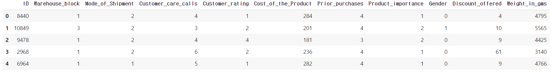
→ 명목형 변수의 컬럼명들을 cols 변수에 담고 반복문을 사용해 LabelEncoder() 작업을 진행한다.
# trainID 삭제, testID 값만 옮겨둠
X_train = X_train.drop('ID', axis=1)
X_test_id = X_test.pop('ID')
X_test.head()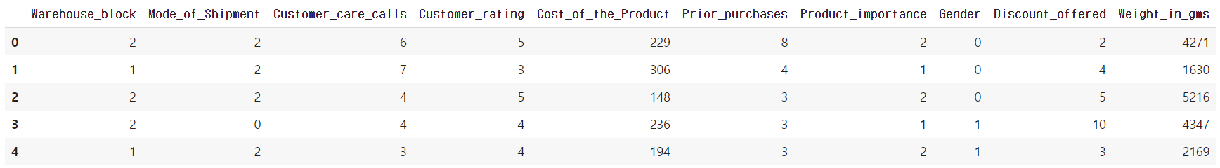
→ 훈련 과정에서 필요 없는 ID 열을 삭제한다.
→ 최종 제출 csv 파일에 사용할 ID열을 X_test_id 변수에 따로 담아둔다.
4. 모델 및 평가
# 라이브러리 불러오기
from sklearn.linear_model import LogisticRegression
from sklearn.tree import DecisionTreeClassifier
from sklearn.ensemble import RandomForestClassifier
from xgboost import XGBClassifier

from sklearn.metrics import roc_auc_score
from numpy.random.mtrand import RandomState
# 검증 데이터 분리
from sklearn.model_selection import train_test_split
X_tr, X_val, y_tr, y_val = train_test_split(X_train,
y_train['Reached.on.Time_Y.N'],
test_size=0.2,
random_state=2021
)
X_tr.shape, X_val.shape, y_tr.shape, y_val.shape
실행 결과 :
((7039, 10), (1760, 10), (7039,), (1760,))→ 로지스틱 회귀, 의사결정나무, 랜덤포레스트, XGBoost 4가지 모델로 예측 후 roc_auc_score로 평가하기 위한 코드
→ X_train, y_train 데이터를 훈련용과 검증용 데이터로 분리한다.
# 로지스틱 회귀
model = LogisticRegression(random_state=2022)
model.fit(X_tr, y_tr)
pred = model.predict_proba(X_val)
print(roc_auc_score(y_val, pred[:,1]))

실행 결과 :
0.7084136003323999
# 의사결정나무
model = DecisionTreeClassifier(random_state=2022)
model.fit(X_tr, y_tr)
pred = model.predict_proba(X_val)
print(roc_auc_score(y_val, pred[:,1]))
실행 결과 :
0.6321275746145835# 랜덤포레스트
model = RandomForestClassifier(random_state=2022)
model.fit(X_tr, y_tr)
pred = model.predict_proba(X_val)
print(roc_auc_score(y_val, pred[:,1]))
실행 결과 :
0.7279225281811363# XGBOOST
model = XGBClassifier(random_state=2022)
model.fit(X_tr, y_tr)
pred = model.predict_proba(X_val)
print(roc_auc_score(y_val, pred[:,1]))
실행 결과 :
0.7348018821599512→ 4가지 모델 중 XGBoost의 예측률이 0.73으로 제일 높게 나온 것을 알 수 있다.
5. 예측 및 제출
# 예측
pred = model.predict_proba(X_test)
pred

실행 결과 :
array([[0.717337  , 0.28266302],
       [0.5674526 , 0.4325474 ],
       [0.7829215 , 0.21707852],
       ...,
       [0.51868916, 0.48131084],
       [0.5928507 , 0.40714929],
       [0.78776836, 0.2122316 ]], dtype=float32)
→ XGBoost 모델에 X_test를 넣어 실행한 결과이다.
→ 왼쪽은 정시 도착 확률, 오른쪽은 정시 도착하지 않을 확률 이다.
# 데이터프레임 만들기
submit = pd.DataFrame(
    {
        'ID' : X_test_id,
        'Reached.on.Time_Y.N' : pred[:,1]
    }
)
→ 문제에서 제시한 형식을 만들기 위해 데이터 프레임에 ID와 정시 도착하지 않을 확률을 넣어 만들어준다.
# 데이터 확인
submit.head()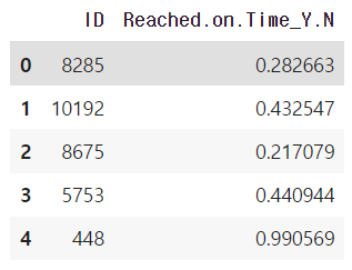
→ 데이터프레임 확인시 ID와 정시 도착하지 않을 확률이 잘 들어간 것을 확인 할 수 있다.
# CSV파일 만들기
submit.to_csv('수험번호.csv', index=False)
→ 제출하기 위한 csv파일을 만드는 코드이다, index는 False로 지정해 생성되지 않도록 한다.
5. 제대로 제출 되었는지 확인
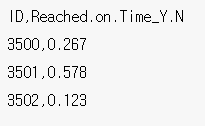
pd.read_csv("수험번호.csv")→ 생성한 csv 파일이 제대로 만들어지고 제출되었는지 read_csv로 불러와 재확인한다.
6. 채점 (수험자는 알 수 없는 부분)
you = pd.read_csv("수험번호.csv")
print("당신의 score는?:",roc_auc_score(y_test['Reached.on.Time_Y.N'], you['Reached.on.Time_Y.N']))

실행 결과 :
당신의 score는?: 0.7312431644814588
→ 수험자는 알 수 없는 부분이지만 y_test를 통해 평가 시 0.73 예측률로 나쁘지 않은 성과가 나온것을 확인 할 수 있다.
'빅데이터분석기사 > 작업형2' 카테고리의 다른 글
| [작업형2] 심장마비 확률 높은 사람 구하기(분류 / 튜닝) (0) | 2023.06.17 |
|---|---|
| [작업형2] 에어비앤비 가격 예측하기(회귀) (0) | 2023.06.17 |
| [작업형2] 신용카드 서비스를 떠나는 고객 확률 구하기(분류) (0) | 2023.06.17 |
| [작업형2] 보험가입 확률 구하기(분류) (1) | 2023.06.17 |
| [작업형2] 고객의 성별이 남자일 확률 구하기(분류) (1) | 2023.06.15 |